
NBA Finals prediction using BTL Algorithm
The Bradley-Terry-Luce(BTL) Algorithm assesses the talent of contestants based on one-on-one matches. It uses pairwise comparisons to estimate a single parameter that approximates the latent ability of the contestant. The BTL algorithm is quite versatile, meaning the result of matches can be a subjective ranking or objective like a win\lose\draw scenario, as long as the results are consistent throughout the data. The BTL model assumes that the probability of team \(i\) beating team \(j\) (\(i \triangleright j\)) will depend on their latent abilities.
\[p(i \triangleright j | \alpha) = \sigma (\frac{\alpha_i - \alpha_j}{scale})\]where \(\alpha\) is the \(T \times 1\) latent ability vector, \(\sigma(x) = \frac{1}{1+e^{(-x)}}\) is the sigmoid function and \(scale\) is used as a normalizing term for rankings. Basically, under this model, higher the difference between the latent ability of team \(i\) and team \(j\), higher the probability of team \(i\) beating team \(j\).
When dealing with single player contestants, it is easy to link different aspects of the player into a single latent ability parameter with simple assumptions, but when teams are considered this task is relatively harder. In our scenario, for example, changes in team roster, player injuries & rest days and team chemistry all play a role in a teams performance and therefore affect the latent ability of the team. In order to account for these, a posterior latent ability vector was used and some assumptions were made:
- Team records - dichotomous outcome(win\lose) - are the talent indicator; i.e. score marigins are omitted.
- Temporary changes in team rosters - rested, suspended players - does not alter the overall team talent
- Team chemistry, player usage and coaching effects are omitted.
To get the posterior latent ability vector of teams, first we need to establish a prior distribution. This was done by using the 2015-16 Regular Season records and to account for trades between teams, the difference in Real Plus\Minus(RPM) values of traded players were added1. For example, for Chicago Bulls the prior latent ability:
\(\alpha_{CHI}^{15-16} = Wins_{CHI}^{15-16} + \Delta TotalRPM^{16-17}\).
We can then define the game data matrix \(M^{16-17}\) and using this with our derived prior distribution we can get the posterior latent ability distributions of teams before they enter the playoffs.
\[p(\alpha|M^{16-17}) \propto p(M^{16-17}|\alpha)p(\alpha^{15-16})\]In a regular season, each one of the thirty NBA teams plays 82 games with each other and the number of games Team A plays with Team B depends on their conferences. Each team plays 3-4 games with same conference teams (each conference has 15 teams, a given team plays 4 games with 10, and 3 games with 4 same-conference teams) and 2 games with other conference teams. For example, Chicago Bulls played 4 games with Cleveland Cavaliers and 2 games with Golden State Warriors in 2016-17 Regular Season. So, the regular season provides a useful dataset that can be used in a BTL implementation, since each team plays with each other at least 2 times2.
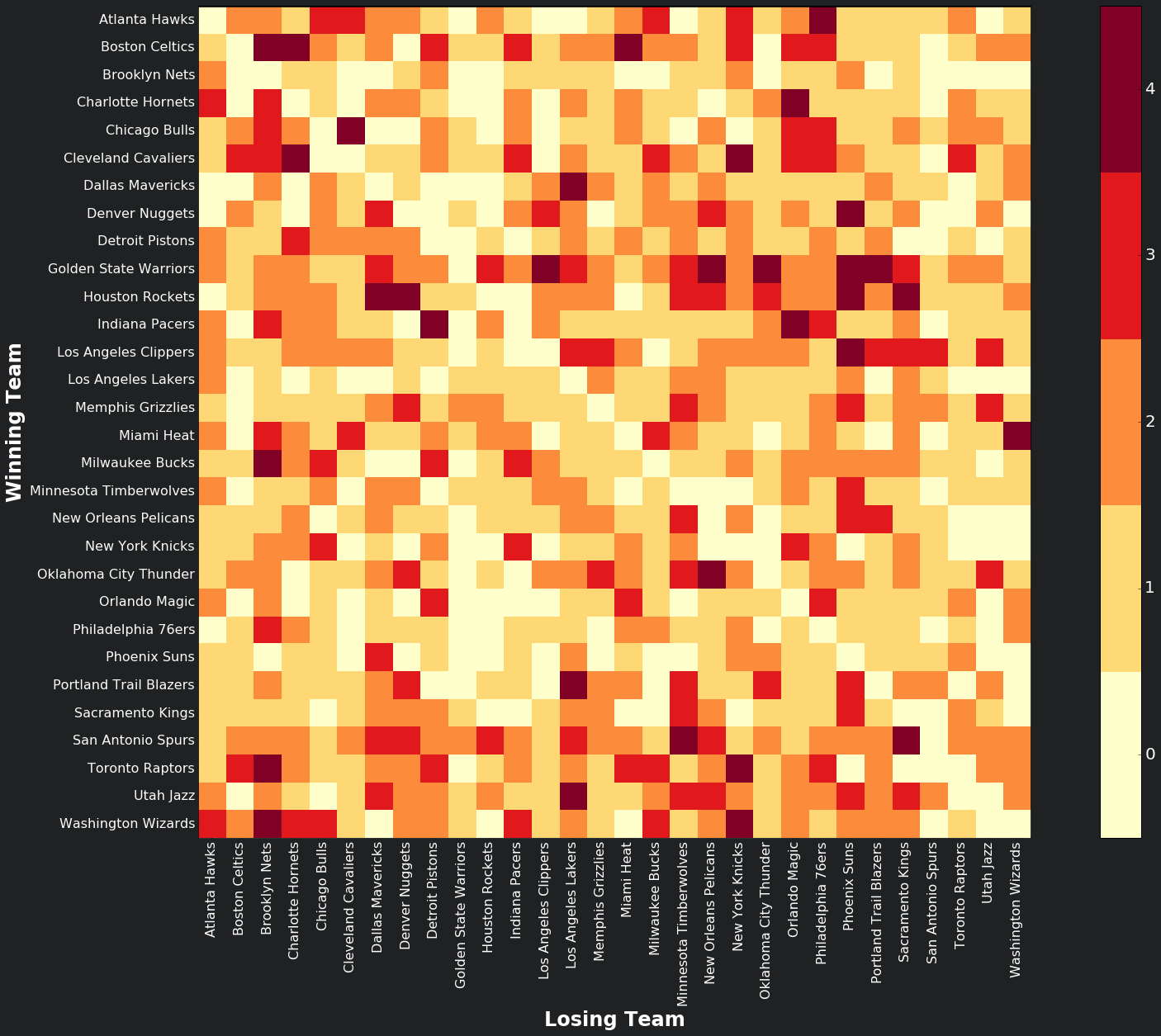
Scraping the 2016-17 season standings from here, and mapping them onto a grid, where the y-axis is the winning and the x-axis is the losing team, we get a match result matrix, \(M^{16-17}\), where darker shades indicate high number of wins against the other team. As expected the values in the diagonal of the matrix are zero.
The maximum likelihood of the model is given by:
\[p(M^{16-17}|\alpha) = \prod_{ij}[\sigma(\alpha_i-\alpha_j)]^{M_{ij}}\]where \(M_{ij}\) indicates the amount of times team \(i\) beat team \(j\).
To get a distribution of each teams latent talent, not the talent difference between the teams but the the talent difference compared to the scaling factor - 82 in NBA case - is used. \(\alpha^{league}_i\) in this case is all the possible victories team \(i\) can get:
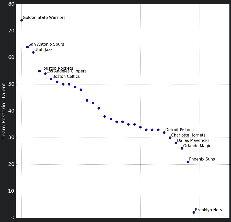
\[L \equiv \log p(X|\alpha) = \sum_{i,j} M_{ij}\log\sigma(\alpha^{league}_i-\alpha_j) + M_{ij}\log(1-\sigma(\alpha^{league}_i-\alpha_j))\]taking the exponential of the result will then give us a team talent distribution, which we will randomly pick from.
Below are all the picked talents:
After acquiring the posterior talents of all of the teams, we can use the talents of the teams that made it to the playoffs and implement an iterative process that matches the teams and simulates the series games by:
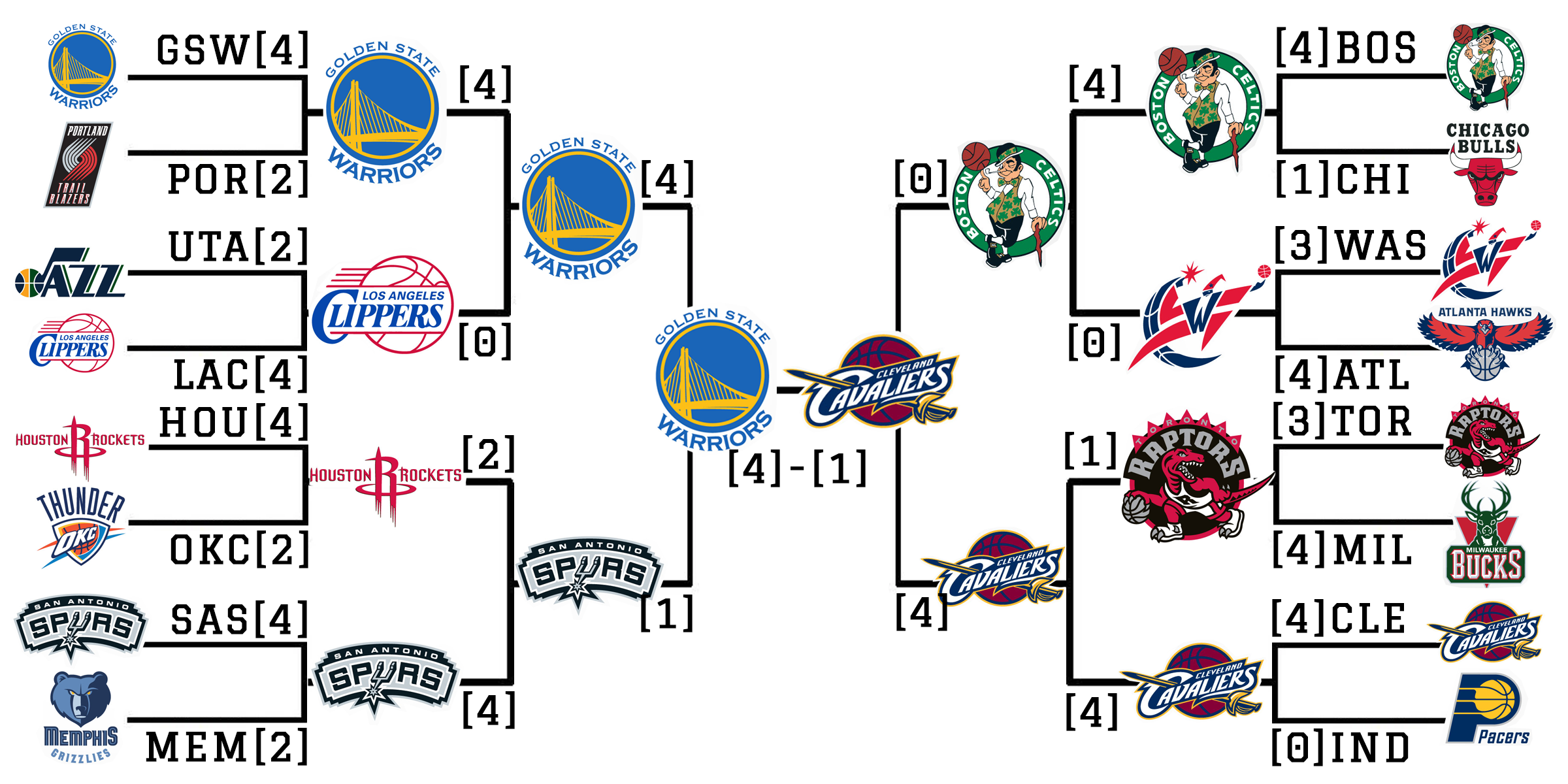
\[p(i \triangleright j | \alpha) = \sigma (\frac{\alpha_i - \alpha_j}{scale})\]The simulation can sometimes give unexpected results, because it treats each game as an independent occurance. This is a gross misrepresentation of NBA playoff series as each game heavily depends on previous games and home court advantages. Even though, after running the simulation several times, the results are generally in alignment with found latent talents of teams and Golden State Warriors plays NBA Finals most of the time.
All in all, we can confidently say that we predicted the 2017 NBA Finals pretty accurately as it can be seen below, and yes cherry picking was used to obtain this result.
This was a final group project done with my friends Onur Alten and Feyzullah Alim Koyuncu.
1 - The RPM values for a player depends on the team he plays, so the added RPM value of a player is actually his effectiveness when he was in his previous team. Further information about the derivation and indication of Real Plus\Minus values can be found here
2 - It should be noted that in situations where every team plays with each other - like NBA - it is rather intuitive to figure out the latent ability of each team by simple observation. The BTL algorithm will be more useful in situations where each team does not play with each other; e.g. the NCAA.